Now what is VAE….VAE is basically Variational Autoencoders which was actually built on the limitations of normal Autoencoders.
Let me give you a summary on what an Autoencoder is.
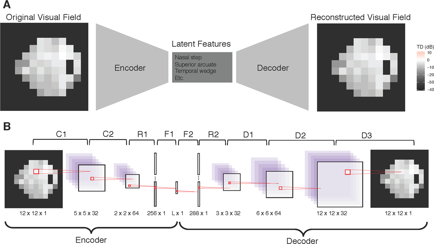
It consists of an encoder, a decoder and finally a bottleneck which is used to compute something called the latent space.
What is latent space? Think of it as a compact box where the encoder stores the most useful features of the input — a compressed representation.
The autoencoder’s role is to take an image as input, the encoder extracts useful features, the bottleneck retains those features and the decoder tries to recreate the same image from the bottleneck. The reconstruction error (e.g., mean squared error) tells us how well the autoencoder learned to preserve important information.
From Autoencoders to Variational Autoencoders
A plain autoencoder learns a deterministic mapping: input → bottleneck vector → reconstruction. VAEs make the bottleneck probabilistic. Instead of storing a single point, the encoder outputs parameters of a probability distribution (usually a Gaussian) over latent variables. At training time we sample from this distribution and pass the sample to the decoder.
Why? Because treating the latent space as a distribution gives two big wins:
- It regularizes the latent space so similar inputs map to nearby distributions, which makes interpolation and generation smooth.
- It turns the model into a proper generative model: we can sample from a simple prior (e.g., standard normal) and decode to get new, realistic examples.
Latent distributions and sampling
The encoder produces two vectors: a mean and a log-variance. These define the Gaussian
and feed z to the decoder which tries to reconstruct x.
Naively sampling inside the network would break gradient flow. The trick that fixes this is the reparameterization trick: instead of sampling z directly, we sample and compute
This operation is differentiable with respect to mu and sigma, so we can train the whole model with backprop.

Training objective: ELBO (in short)
The VAE is trained to maximize a lower bound on the data log-likelihood, commonly called the Evidence Lower Bound (ELBO). For each input x, the ELBO decomposes into two terms.
log p(x) >= E_{q(z|x)}[log p(x|z)] - KL(q(z|x) || p(z))
The first term is the expected reconstruction log-likelihood and the second is the Kullback–Leibler divergence that pushes toward the prior.
Maximizing the ELBO balances reconstruction quality and how close the latent distributions are to the prior. If the KL is too small, the model ignores z; if it’s too large, reconstructions suffer. In practice you often see a weighted KL term to trade off disentanglement and fidelity.
Minimal PyTorch VAE (snippet)
import torch
from torch import nn

class SimpleVAE(nn.Module):
    def __init__(self, latent_dim=32):
        super().__init__()
        self.encoder = nn.Sequential(
            nn.Flatten(),
            nn.Linear(28*28, 400),
            nn.ReLU(),
        )
        self.fc_mu = nn.Linear(400, latent_dim)
        self.fc_logvar = nn.Linear(400, latent_dim)

        self.decoder = nn.Sequential(
            nn.Linear(latent_dim, 400),
            nn.ReLU(),
            nn.Linear(400, 28*28),
            nn.Sigmoid(),
        )

    def reparameterize(self, mu, logvar):
        std = (0.5 * logvar).exp()
        eps = torch.randn_like(std)
        return mu + eps * std

    def forward(self, x):
        h = self.encoder(x)
        mu = self.fc_mu(h)
        logvar = self.fc_logvar(h)
        z = self.reparameterize(mu, logvar)
        x_hat = self.decoder(z)
        return x_hat, mu, logvar

# Loss (reconstruction + KL)
def vae_loss(x, x_hat, mu, logvar):
    recon_loss = nn.functional.binary_cross_entropy(x_hat, x.view(x.size(0), -1), reduction='sum')
    kl = -0.5 * torch.sum(1 + logvar - mu.pow(2) - logvar.exp())
    return recon_loss + kl
- Anomaly detection (low-likelihood reconstructions indicate anomalies)
- Conditional generation and semi-supervised learning (with slight extensions)
If you want, I can also add a tiny training loop example for the snippet or generate a larger, annotated diagram for the post.