We’re at the midterm mark of Google Summer of Code, which means it’s time to stop and look back at what actually got built. I put together a “Work Done Till Now” presentation for the evaluation, and instead of letting those slides quietly die in a Google Drive folder, I figured I’d turn them into a proper post.
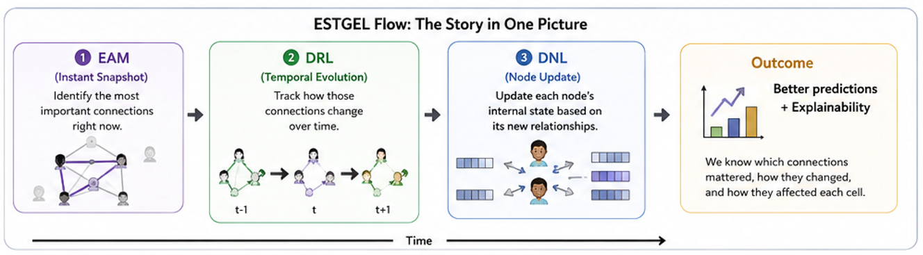
So here’s the honest tour week by week, what I started with, what broke, and where things stand now. The project, if you’re new here, is ESTGEL (Enhanced Spatial-Temporal Graph Edge Learning) for OpenWorm: a graph neural network that watches a C. elegans embryo develop cell by cell and learns which cell-to-cell interactions actually matter.
Week 1 Getting eyes on the data
Before you can model anything, you have to see it. Week 1 was all about turning the raw EPIC microscopy data into something I could actually look at and reason about.
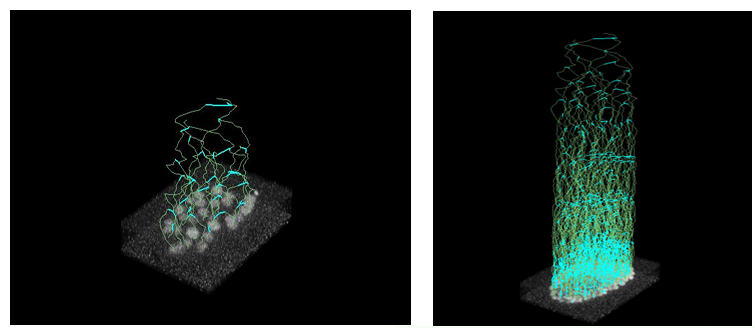
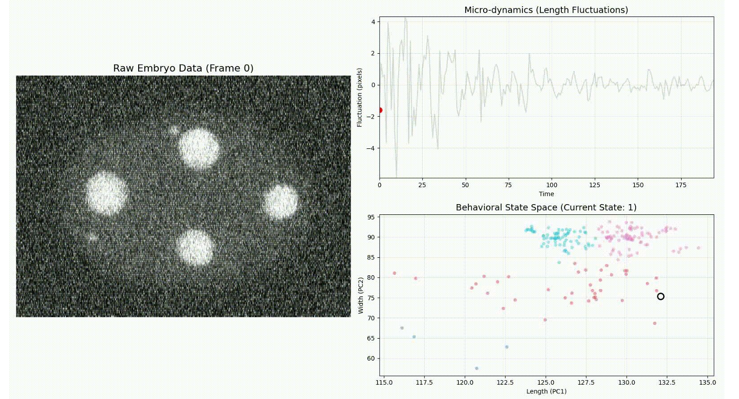
The embryo data starts life as a noisy volumetric scan a cloud of blobs where each blob is (hopefully) a nucleus. I built out the first visualizations: 3D reconstructions of the tracked cells over time, the raw embryo frame at t=0, and a couple of exploratory plots to get a feel for the dynamics. The “micro-dynamics” plot tracks length fluctuations over the timeline, and the behavioral state-space plot projects each frame down so you can watch the embryo drift through different states.
None of this is the model yet. But it’s the part that tells you whether your data is even trustworthy and it caught a few things early.
Week 2 Building the dataset loader
Visualizations are fun, but the model needs a clean, consistent stream of tensors. Week 2 was the unglamorous but essential work of writing the dataset loader.
The loader takes each embryo CSV and returns a spatio-temporal tensor plus an alive_mask that tracks which cells actually exist at each timestep (cells are born as the embryo divides, so the count is not constant). A single sample came out shaped like [710, 5, 220] that’s 710 nodes, 5 features per node, across 220 timesteps with an alive_mask of [710, 220].
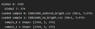
The bigger win was making it handle multiple embryos with different lengths and node counts and align them into a shared global frame:
Global N: 2769
Global T: 374
Loaded sample 0: CD011505_end1red_bright.csv (t0=1, T=374)
Loaded sample 1: CD011605_5a_bright.csv       (t0=1, T=374)
  sample_0 x shape: [2769, 5, 374]
  sample_1 x shape: [2769, 5, 374]
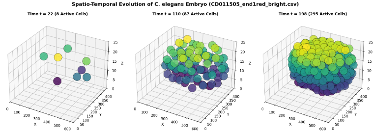
To sanity-check it, I rendered the spatio-temporal evolution of an embryo directly from the loader’s output from a handful of active cells early on to a couple hundred packed together by the end. If the loader is wrong, this plot looks wrong, so it doubled as a test.

Week 4 Training the ESTGEL classifier
With the data flowing, Week 4 was about wiring everything into an actual training loop and getting the first real numbers out.
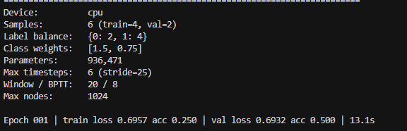
The setup was deliberately small so I could iterate fast the goal was a working pipeline, not a leaderboard score:
Device:        cpu
Samples:       6 (train=4, val=2)
Label balance: {0: 2, 1: 4}
Class weights: [1.5, 0.75]
Parameters:    936,471
Max timesteps: 6 (stride=25)
Window / BPTT: 20 / 8
Max nodes:     1024
The model is a ~936K-parameter graph network, trained with class-weighted cross-entropy to deal with the imbalance between the two phenotype classes, gradient clipping, and truncated backprop through time so the temporal unrolling stays tractable.
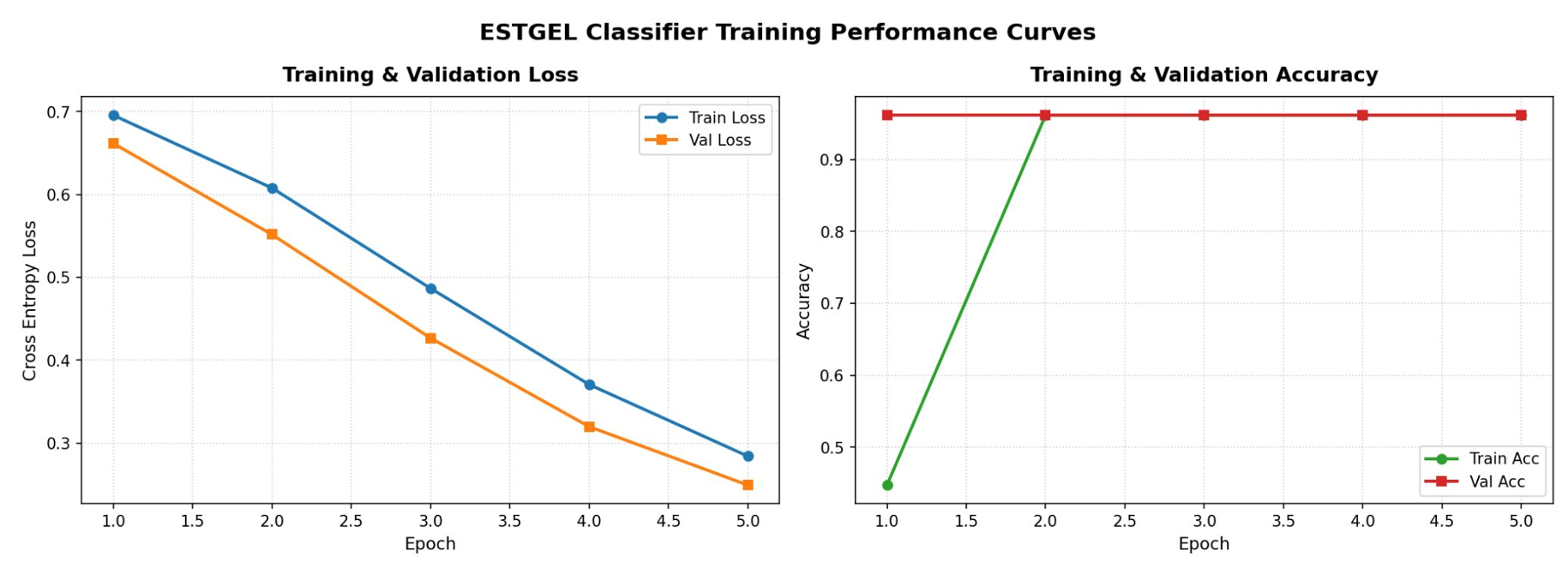
The first smoke test started exactly where you’d expect a randomly-initialized model to start around 50% and then the loss curves came down cleanly:
Epoch 001 | train loss 0.6956 acc 0.447 | val loss 0.6616 acc 0.962 | 378.5s
Epoch 002 | train loss 0.6078 acc 0.962 | val loss 0.5516 acc 0.962 | 299.3s
Epoch 003 | train loss 0.4866 acc 0.962 | val loss 0.4266 acc 0.962 | 302.4s
Epoch 004 | train loss 0.3705 acc 0.962 | val loss 0.3197 acc 0.962 | 305.4s
I want to be honest about what this does and doesn’t mean: with six embryos, that 0.962 validation accuracy is a “the plumbing works” result, not a “we’ve solved developmental biology” result. What matters here is that loss decreases smoothly on both train and validation, nothing explodes, and the whole forward → loss → backprop → checkpoint loop runs end to end. That’s the foundation everything after this stands on.
Week 5 Reading the attention
A classifier that says “control” or “perturbed” isn’t that interesting on its own. The whole point of ESTGEL is the edges which cell-cell interactions the model leans on to make that call. Week 5 was about pulling those attention weights back out and making them legible.
I extracted the top cell-cell attention weights across the developmental timeline for a wild-type (WT) embryo. Early on there are only a handful of active connections; by the later timesteps there are hundreds. Walking the timeline, you can watch specific lineage interactions light up:
- t=030 (8 active connections):
ABal → ABala,ABal → ABalp,ABar → ABara(weights ~1.0) - t=090 (58 active connections):
ABalpap → ABalppa,ABarpap → MSpaa,Epr → Cpa - t=150 (285 active connections):
ABalaaal → ABalaaaar,ABplpaaap → ABalpaapp
Then the more interesting bit: I compared attention in the control (WT) embryo against an RNAi-perturbed one. For a given interaction, the spatio-temporal attention profile over developmental time looks different between the two conditions a peak that shows up in WT can flatten out under RNAi, or shift to a different window entirely. That contrast is exactly the kind of signal that makes this model worth building: it’s a handle on when and where a perturbation changes the embryo’s internal wiring.


Week 6 The embryo development dashboard
All of the above lived in scattered scripts and notebook cells. Week 6 pulled it together into something you can actually use: an interactive Embryo Development Dashboard a spatio-temporal GNN and explainability explorer.
On the left there’s a phenotype selector (Control vs Perturbed), a timeline scrubber, and live readouts active nodes, active edges, average attention weight, and the current top-5 cell-cell interactions. The centerpiece is a 3D spatial map of the embryo where cells are rendered as nodes you can rotate and zoom, with the ESTGEL attention scores driving what’s highlighted. Along the bottom sit the embryo growth profile (WT vs RNAi) and the attention-contrast plot, both synced to whatever frame you’re scrubbed to.
This is the moment the project stopped feeling like “a model that outputs numbers” and started feeling like a tool a biologist could sit down with.

On to the next steps what do we have?
Midterm is a checkpoint, not a finish line. Here’s the rough plan for the back half:
Week 9 Tool building & visualization. Build out the visual pipeline properly: render cells as nodes in 3D space and use the ESTGEL attention scores to visually highlight the most critical edges driving development. Leave a buffer for pending cleanup.
Weeks 10–11 Integrate the temporal data and scores. Tightly integrate these new D-GNN modules into the larger DevoLearn / DevoGraph pipeline, and add interactive functions so users can trace decision paths and analyze critical spatio-temporal hotspots.
Week 12 Final wrap-up. Documentation for the new functionality, a report for the final evaluation, and of course a blog about the newly added tools.
That’s the state of things at the halfway point. The unglamorous foundation (loader, training loop, checkpointing) is in place, the model runs end to end, and the attention maps are already surfacing biologically-shaped signal. The second half is about turning that from “it works” into “people can use it.”
More soon.